Dashboards, Scorecards & Visualization

The following data visualization has four buttons for audiences to select different years:

https://flowingdata.com/2016/06/28/distributions-of-annual-income/

Last lecture we talk about the if we need to use interactive data visualization to make our point. In my opinion it depends on the case, and i do not think too much interactive things are helpful. Take the above visualization for example, the author only give four choices: 1960, 1980, 2000, 2014. Also, the data visualization has animations when user switch years. The animation plays an important role in this visualization because we can see and compare the amount changes between different majors. I find it super fun to play with this data visualization even though it has four choices.

So, my conclusion is, as long as the interactive data visualization can give use an idea about the difference between selections, it is a good visualization.

Also, I found an article about how to make interactive data visualization successful. Maybe I will table about it int the next blog post.

http://www.forbes.com/sites/benkerschberg/2014/04/30/five-key-properties-of-interactive-data-visualization/#eb593ab44eb0

Rules to keep in mind to devise a strong argument:

Claim is the point an arguer is trying to make and wants another to accept. When a claim is made, the question to be asked is “What is your point?”

Example: The Ravens will win the Super Bowl this year.

Visualization refers to the proof or evidence an arguer offers.   Grounds answers the questions, “What is your proof?”. It can consist of statistics or reports via physical evidence of reasoning.

Example: They have the best defense in the league.

Warrant is the inferential leap that performs a “linking” function by establishing a mental connection between the grounds and the claim

Example: The team with the best defense usually wins.

Backing consists of evidence to support the type of reasoning employed by the warrant.

Example: The team with the best defense has won each of the last five years.

Qualifier states how sure the arguer is about his/her claim

Example: The probability that the Jets will win the Super Bowl is 80 percent.

Rebuttal admits to those circumstances or situations where the argument would not hold.

Example: Anything could happen. The Ravens defense might have a lot of injuries.

Reference: http://commfaculty.fullerton.edu/rgass/toulmin2.htm

Data will be remembered only if presented in the right way. Often, executives and managers are being bombarded with charts, graphs, dashboards with complex data analytics. The reason why they struggle with the data-driven decision making is that they don’t understand the story behind the data. In this way, a powerful story with data means a lot.

Stories are meaningful when they are memorable, impactful and personal.  When data and stories are used together, they resonate with audiences on both an intellectual and emotional level. To tell a meaningful story, you’d better:

Identify the audience. What does the audience know about the topic? There are usually five types of audience in common: novice, generalist, management, expert and executive. The novice is new to the subject, but doesn’t want to oversimplification. The generalist is aware of the topic, but looking for an overview understanding and major themes. The management want in-depth, actionable understanding of intricacies and interrelationships with access to detail. The expert want more exploration and discovery and less storytelling with great detail. The executive only has time to glean the significance and conclusions of weighted probabilities.

Use data visualization to complement the narrative. There are mainly two visual narrative genres: one is author-driven narrative, which doesn’t allow readers to interact with charts; the other one is reader-driven narrative, which provides ways for reader to play with the data. Those two should be balance intended by author with story discovery on the part of reader. A good data visualization should stands on its own. If you take it out of the context, the reader should be able to understand what the chart is saying as well. A good data visualization also should be easy to understand. while too much interaction can be distractive, the visualization should incorporate some layered data so the curious can explore.

Reference: https://www.thinkwithgoogle.com/articles/tell-meaningful-stories-with-data.html

Bubble charts give you the ability to visualize up to 4-dimensions of data and are an absolute fan favorite! They communicate the count or proportion of a variable where the size of the bubble reflects the quantity in two dimensions. We could add the third dimension by plotting the different sized bubbles with x and y axis like a scatter plot. The fourth dimension is added usually by use of different colors (shades of a color) to sort data into categories.

The bubble chart shows a lot of data all at once, making it tricky and hard to understand the answer on the first go. The difficulty is in interpretation of bubble graphs. While they can give a quick comparison of values by looking at them, they are not as well suited for accurate determination of analysis of your data.

Best practices for Bubble Charts:

1. Use when the audience is aware of the data and educated.
2. Size bubbles appropriately.
3. Do not use when data results in overlapping bubbles.

As we can see in the chart, there is total chaos and it creates a piece of modern art, with multiple perceptions at the user end. With no prior information on what data is being represented there is no clear understanding of the details and requires additional effort to decipher and generate an analysis. Hence at times bubble charts are as useless as pie charts.

 

http://www.quickbase.com/quickbase-blog/when-to-use-bubble-charts-to-display-your-data

https://visage.co/data-visualization-101-bubble-charts/

http://www.msktc.org/lib/docs/KT_Toolkit/Charts_and_Graphs/Charts_Tool_Bubble_508c.pdf

 

Manipulation of the facts or deception of the reader can be both intentional and unintentional. The data would be distorted which lead to misleading to audience. There are several ways to present misleading visualizations.

1.Truncated Axis.

2. Area as quantity.

The two graphs above allures the audience to feel that the difference in percentage is huge.

3. Aspect Ratio.

The aspect ratio of the chart has been distorted by stretching the X-axis, which mislead the audience to feel the change was not significant by the flattened line.

4. Inverted Axis

The Y-axis has been inverted, hence, creating an illusion that the access to safe drinking water has declined.

This visualization is extremely interesting with good aesthetics. As was discussed in class last week, this visualization covers most of the important aesthetics concepts such as getting it right in black and white (almost), no unjustified 3D and resolution over immersion.

Facebook worldwide friendships mapped

However, it is not as simple as it looks like. A lot of background analytics have gone into consideration before preparing this visualization. Let’s see how to decipher this.

Firstly, weights were defined for each pair of cities as a function of distance and the number of friends between them. Then the cities with were connected using the count of number of friends. The cities with the most friendships between them have been drawn on the top of others. The color ramp has been beautifully used so that the lines are created depending on the weights; which also means that the stronger the connections, the lines would be more visually prominent.

However, there are some fundamental problems with this visualization. Firstly, there is no legend or text representing what the visualization is all about. There should be a mechanism for the audience to know what it wants to assert basis the color, thickness and degree of shading of the connected lines. Secondly,  few areas on the map show no lines and is dark. This may be due to the fact that Facebook has not reached those locations or the usage is not prominent in such countries or the data is unavailable for all such locations; which is not clear from the infographic.

The visualization could be improved by making it more interactive. A highly visual dashboard like this should enable the audience to perform basic analytical tasks such as drill down and examine the underlying data. For example, if one wants to zoom in and see the number of the friendships within the country or with another particular country; one should be able to do that.

Recently President Trump released an executive order to ban immigrants from seven countries. This visualization is simple yet powerful in conveying how it will impact the immigrants who already are living in USA and what is their education, salaries, etc.

Demographics for immigrants from banned countries

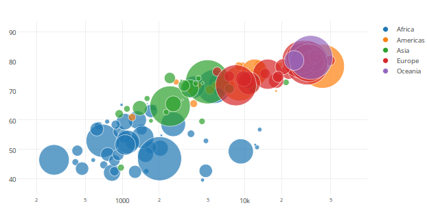
The immigrants from these seven countries constitute to about 2% of the total population of USA. The dashboard shows the percentage of the immigrants and their level of education and comparing them to the US national average. It can be seen that immigrants from Iran, Libya and Syria with advanced degrees is higher than the US national average in this domain.

Further analysis shows that residents from Iran and Syria are more likely than the population to be engineers, managers and teachers. These immigrants are also scattered in almost every state. With the US Median salary for such blue collar jobs is $54,645 pa; the salary of Iranians in the same job bracket is over $65,000. 

The dashboard also shows that the figures for Iran residents is higher than the other six banned countries, because the number immigrants from Iran prospered from 1980’s to 2010, which means that the higher the number of immigrants; higher with be the absolute number of managers, engineers and people holding blue collar jobs. As discussed in lectures, in this case, enumerating the figures in ‘percentage’ or ‘average’ is a better representation of these statistics.

Further, the representation of now-citizens has been appropriately depicted in percentages, most immigrants have now become residents of the United States. Further, about 10,000 of these immigrants have also served in the US Army. Also. the residents are also scattered geographically, with no specific area of concentration.

As per news reports from NY Times, more than 856,000 people have been affected by this ban but only 3 of countries were known to be in violent attacks since 2001.  Most accused have been from countries not listed in the ban and many were born in the United States.

We will have to wait and watch on how the ruling will actually affect the immigrants, visa holders and permanent residents.

Today’s blog is about the real time information about the traffic and web attacks worldwide.

This activity is performed by a company called Akamai. It constantly monitors the internet conditions on these two parameters worldwide and presents on the graph real time.

https://www.akamai.com/us/en/solutions/intelligent-platform/visualizing-akamai/real-time-web-monitor.jsp

These two graphs serve the following purposes:

• Monitoring greatest web traffic
  
• Cities with the slowest web connections also known as latency
• Geographic areas with the most web traffic also known as traffic density

This visualization is interactive and one can look at the network traffic and attacks country wise.

Analyzing this visualization, one can observe that the highest network traffic is in the UK and European subcontinent. However, the maximum number of attacks is in California with an average of 1,423,212 attacks per 24 hours.

However, it seems like this monitoring tool focusses on only certain areas and does not provide a comprehensive overview of the attacks in countries like Canada; South American and African countries. Further, no information is available for the network traffic in the Indian subcontinent. This does not mean that there is no network traffic in those areas but it means that the comprehensive data is not available for all the countries.

This is the graph showing valuation of Facebook, Inc. Though it is simple bar graph you can identify many problems in this visual.

http://blogs-images.forbes.com/naomirobbins/files/2011/11/press-005-021.jpg

The very first thing you will find is the truncated vertical axis. Normally we judge values of the bars in the bar graph by its length. Here the second bar appears to be twice as high as of the first bar. One can conclude that valuation is doubled from December to January. Every bar graph needs a zero on its scale.

Second, the horizontal axis is evenly spaced but dates are confusing the reader. There is one bar for December, one for January, none for February, two for March, and so on. Therefore, the trend that results from following the top of the bars is distorted. Mainly, the high valuation of $84 billion appears to hold for a long period, when in fact the total time at this value was less than a month (June 22 to July 19).

Last thing is excessive use of dollar sign on the vertical axis and on data labels. Instead of showing it twenty times in graph, they could have mentioned the scale as ‘dollar units’. These are not serious problems but it does give misleading information.

Source: http://www.forbes.com/sites/naomirobbins/2011/11/17/whats-wrong-with-this-graph/#7acf99f199d4

 

The following graph is from Bloomberg (2013); which for many is a trusted source. Unfortunately, even this trusted source has misused power of statistics to deceive people.

Looking at this graph, a common man would be highly concerned with the slope depicting sharp decline in median income for U.S. men but in true sense there are more flaws with the graph than with the fact depicted.
The first flaw is regarding incomplete information. The designer has only shown 2 data points and no information is depicted about what happened in middle years. On investigating more from U.S Census data one can see that median income was actually stable between 1972 and 1999 which is contrary to what designer has depicted. Also, for age 45-54 there was actually an increase in median income till 2000 and only after that there was a decline in the income.

The second flaw is with the y-axis. The designer has deliberated truncated the y-axis so as to magnify the gap. If the same graph is seen making y-axis start from zero, the decline doesn’t feel much and our perspective about the problem changes.

Lastly on investigating on the data more, we find that from 1947 to 1972 there was steady increase in median income and since 1972 (end of Gold standard) there has been a slow decline in the number. The designer has deliberately chosen 1972 and 2012 to catch attention of its readers. The same news can be changed to “Income for men has risen” by giving 1947 and 2012 as new data points.

References:
Image & Article Source: https://www.bloomberg.com/news/articles/2013-12-31/for-u-s-men-40-years-of-falling-income
Other Source: https://medium.com/i-data/misleading-with-statistics-c63780efa928#.qaw475rwg