Author: vinamrata

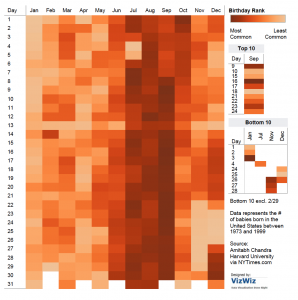
When we see innovative charts, it looks attractive and beautiful. But then we think is it necessary to put so much efforts into one chart which could have been communicated in simple way? Here comes the question of communicating your message and engaging the user to explore the story.

http://graphics.wsj.com/infectious-diseases-and-vaccines/

From the above link, heat maps show the result of vaccination over diseases like Polio, Measles, Hepatitis A. We can see there are lot of efforts taken to create such a colorful and attractive visualization to convey a message that ‘Vaccination eradicated serious diseases.’

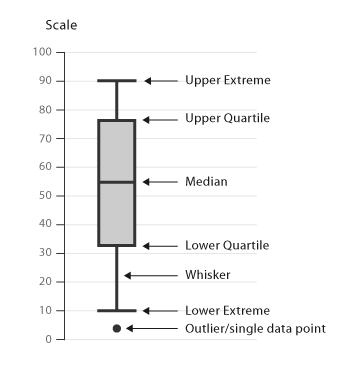
Instead of this heat map they could have used line chart as shown in figure below.

https://www.statslife.org.uk/images/significance/2016/graphs/Vac-Figure-8.png

Saying it should have been a line chart forgets two important aspects of communication which are sometimes as important as complying with the “rules” of data visualization.

Data storytelling can be beautiful as well as functional.

So far we have seen many charts. What comes to your mind when you see heat map? I think this a novel and interactive design delighted with the density of data which you can further explore. And the impact of vaccination was clearly displayed. Simple line chart also conveys the same message but beauty and functionality together achieve more.

The perfect chart does not exist.

When you have rich dataset, story can be told in different ways. Instead of saying what a chart should have been, we should explore what other stories the dataset could say. This doesn’t make one version right or wrong, it just shows new perspectives.

Underlying thought is, “Use data visualization to create ideas not truths” said by Enrico Bertini, assistant professor at the NYU Tandon School of Engineering.

Source: http://www.computerworld.com/article/3048315/data-analytics/the-inevitability-of-data-visualization-criticism.html

This is the visualization based on the survey conducted by the government about American Time Use. It shows how people spend their days means exactly at what time they work.

I found this interesting mainly because of the use of interactivity. Also, the distribution of work schedule is rightly displayed by histogram. Using two filters user can analyze how much is the difference in work schedules for different occupations.It seems overcrowded at first sight but use of highlighters and shading have made it easy to perceive.

We can see most of these occupations fall under conventional work shift 9 a.m.- 5 p.m. But emergency services (police officers, fire fighters) have higher share of work till midnight.

Another interesting thing is we can see who takes lunch break most seriously and who are workaholic. And obviously, this is peak time for chefs and food services.

I think this graph can be made more appealing if it shows comparison between countries as well. That will be interesting to know cultural differences in work time. Another limitation of this data is for white collar work, the line between life and work can be blurred. For example, lunch or dinner with client can be considered as part of work. This throw a wrench into how work hours are measured overall.

Source: http://www.npr.org/sections/money/2014/08/27/343415569/whos-in-the-office-the-american-workday-in-one-graph?/templates/story/story_php=

In last exercise, we introduced interactivity in our visualization by creating parameters, applying filters, creating sets, calculated fields etc. We had different approaches to make it interactive in what sense. I found this article and would like to share some useful ways in which interactions can be used.

1. Highlighting and Details on demand: Making use of highlights helps user to focus on important part of the visualization. Instead of including all information at once you can allow audience to choose and get details of their interest.

2. User-driven Content Selection: With interactive visualization you give user an ability to change the content and drill down to grab relative information. Such a configurable visualization becomes the template through which different structurally similar data sets are displayed, and additional controls allow the user to change what data gets displayed. When used in such a manner, an interactive visualization can make a much larger data set accessible than a comparable static graphic.

3. Multiple Coordinated Visualization: When you use single graphical representation, it limits number of dimensions. For example, maps emphasize geographic location and timelines the flow of time. Those commonly used representations also often have well-known interactions such as pan and zoom for maps. By assembling multiple standard parts and coordinating them, you can show different aspects of the data set at the same time. Also using appropriate filters user can understand relationships among the data.

4. User-driven Visual Mapping Changes: You can improve the interactivity by showing data in different ways. Allowing the user to reconfigure the mappings from data to visual form (visual mappings) for a fixed visualization type is an alternative that can help in maximizing the visualization size.

5. Integrating User’s Viewpoint and Opinions: In interactive visualizations, you can allow users to enter their opinions and improve their satisfaction with the visual.

Please visit the following website and get better understanding with the given examples.

Source: http://www.scribblelive.com/blog/2012/08/06/interaction-design-for-data-visualizations/

Donut chart shows relationship of parts to a whole but it is important to think if it makes any sense. Just because it looks cool, most of the times it doesn’t tell you much. It depends upon what you want to convey. For example, if it is related to gender ratio or performance of one entity overall, then donut chart will be the best fit. But if you have many entities to display then it may become chaotic.

Image-Source: http://payload.cargocollective.com/1/2/73104/1481815/Pie-Labeled.jpg

The above donut chart displays food consumed in 2010. It is eye-catching, labeled properly with different colors. I would like to comment over some of the issues with this donut chart.

• When you look at each food product you can get its percentage contribution. But it is hard to compare them with each other. You cannot identify minute differences. The contribution of Veggies and Pasta looks similar but there is difference of ~3%. This can mislead the results. While comparing, user has to remember the values for each item causing inconvenience.
• Use of different colors is confusing the user especially for color-blinds. It is hard to distinguish Soup, Salad, Fries and Sushi. They all look same.
• Lower values are not visible at all (Salad, Sushi).

It is possible to transform this messy donut chart into meaningful graph. Simple bar chart will be the better alternative in this case. User can easily identify items and compare the values. No need of color palettes in this case. Bars are easily distinguishable. For the lower values, you can combine them together in one item as ‘other’. If you want to use color palettes, then you can even make categories as ‘Fast-food’, ‘Veggies’, ‘Meat’.

While creating a visualization, we should find to make something that looks cool but does not sacrifice a bit of analytical clarity!

Source:

http://payload.cargocollective.com/1/2/73104/1481815/Pie-Labeled.jpg

http://www.datarevelations.com/with-great-power-comes-great-responsibility-or-think-before-you-use-a-donut-chart.html

 

 

Here is the dashboard representing number of Oscars presented since 1929 (when it was started) till 2014. There is no such strong claim to make from this visualization but instead of just staring at list of Oscar winners, you can play with it for different categories and ratings for each year.

Dashboard: http://www.antivia.com/decisionpoint-excel/samples/oscars.htm

Good things about the visualization:

• Less is more. The dashboard is simple and clean with two bar graphs and a block calculating percentage distribution.
• Right choice of idiom. If we want to find what category of films has highest Oscars then bar graph is best suitable. And it is sorted by the number of winners which grabs users attention to the top category of film.
• Effective use of filters. When it comes to movie, we have different categories, genres, artists, ratings, release year. All of these characteristics are included in this dashboard using filters.
• Information follows the inverted pyramid. The most important and substantial information is at the first view followed by significant details by applying filters and then general background information.
• The percentage calculation for each category gives performance of each category with respect to all categories.

Improvements:

• They could have represented trends in each category over those years. For example, how is the demand for documentaries or animated films for each year.
• It has many filters however it would be tedious for user to select all those filters and find the required information.

To conclude with, this provides valuable insights into trends in industry throughout the years which is much better that scrolling through the tables with multiple columns and millions of rows!

Source: http://insidebigdata.com/2015/02/21/visualization-week-ultimate-oscars-dashboard/

 

I personally have never used a box plot because I didn’t know how to use it and when to use it. But when Professor explained in last lecture about average violations per day using box plot, I found it more appealing. Box plots are great way to quickly examine one or more datasets graphically. Of course, you need to know the meaning of all fields on a box plot to understand it. Here is an easy and simple example of how to interpret a box plot.

• Box plot (aka Box and Whisker Plot) plots all data points and splits it into quartiles (Q1, Q2, Q3) and it is represented as a box which goes from first quartile to third quartile.
• The vertical line drawn at the Q2 is median of data set.
• Two horizontal lines extend from front and back of the box are called whiskers. Whiskers often (but not always) stretch over a wider range of scores than the middle quartile groups.
• The extreme points preceding first quartile and  following third quartile are known as outliers.

We can display three common measures of the distribution in data set.

1. Range: It is the distance between two extreme points on a plot. If we consider outliers, then it is between (5) to (95)-> 90. If we exclude outliers, then it is (95-15) 80.
2. Interquartile range: The middle half of a data set falls within the interquartile range. In a boxplot, the interquartile range is represented by the width of the box (Q3 minus Q1). In the chart above, the interquartile range is (80-38) 42.
3. Skewness: We can identify different skewness patterns based on shape of dataset. If the data points are concentrated at the lower end, the distribution is skewed right and vice-versa. If it is evenly split at the median then it is Symmetric.

In Speed Violations example, we can easily identify danger zones which are nothing but those outliers in box plot. Also, our grades distribution on Camino is also a box plot which gives you where your grades stand in overall class grades, what is the average score and how many are above/below average.

I am trying to create a box plot in Tableau, if anybody has already done please share!

Source: http://www.datavizcatalogue.com/methods/images/anatomy/box_plot.png

http://stattrek.com/statistics/charts/boxplot.aspx

 

 

 

 

This is the graph showing valuation of Facebook, Inc. Though it is simple bar graph you can identify many problems in this visual.

http://blogs-images.forbes.com/naomirobbins/files/2011/11/press-005-021.jpg

The very first thing you will find is the truncated vertical axis. Normally we judge values of the bars in the bar graph by its length. Here the second bar appears to be twice as high as of the first bar. One can conclude that valuation is doubled from December to January. Every bar graph needs a zero on its scale.

Second, the horizontal axis is evenly spaced but dates are confusing the reader. There is one bar for December, one for January, none for February, two for March, and so on. Therefore, the trend that results from following the top of the bars is distorted. Mainly, the high valuation of $84 billion appears to hold for a long period, when in fact the total time at this value was less than a month (June 22 to July 19).

Last thing is excessive use of dollar sign on the vertical axis and on data labels. Instead of showing it twenty times in graph, they could have mentioned the scale as ‘dollar units’. These are not serious problems but it does give misleading information.

Source: http://www.forbes.com/sites/naomirobbins/2011/11/17/whats-wrong-with-this-graph/#7acf99f199d4

 

The world is connected through different forms mainly calls, text messages, emails, social networking websites. Among these social networking media has become more popular. There are definitely higher number of people in your “Friends list” than in your contact list. Why? Because, the world is small! Social apps like Facebook, twitter, Snapchat give opportunity to connect and build relations with others irrespective of country, race etc.

I found this amazing visualization created by one of the intern on Facebook’s data infrastructure engineering team. He used R programming to create such a pretty picture. His main curiosity was to know in what locations people have most connections. The boundaries are not visible clearly but we can identify the country/continent. The brightest region are middle-east part of USA and European countries which represent relationship between people living in those areas. The circular arcs which are routes between two points on earth give resonating effect to the visualization.

He used dataset with millions of records of people with their friends list, location etc. He has shared the details of how he came up with this visualization on the following link.

Source: https://www.facebook.com/note.php?note_id=469716398919

Image source:https://www.quora.com/What-are-some-cool-examples-of-data-visualization-done-in-R

Would you like to know the rank of your birthday? Here you can check with this interesting heat map plotted with days and months. It represents the number of babies born in the United States between 1973-1999. (Non-US citizens please ignore your rank!)

Here heat map is the best suitable visualization and it is made using Tableau. Following are some interesting insights.

• If you hover over your birthday, you will see rank and exactly where it stands.
• Along with the rank top 10 and bottom 10 ranks are displayed separately.
• The orange colored palette helps reader to easily distinguish between dates.
• September month has many of the top days where as January is least common.
• Around major holidays, fewer babies are born.

Heat maps are well-suited for visualizing large amounts of multi-dimensional data and can be used to identify clusters of rows with similar values, as these are displayed as areas of similar color.

Source: http://www.vizwiz.com/2012/05/how-common-is-your-birthday-find-out.html

Image-source:  http://public.tableau.com/views/MostCommonBirthdays/MostCommonBirthdays?:embed=y&:loadOrderID=0&:display_count=yes&:showVizHome=no

 

The days are gone for standing on a street and waiting to get the attention of a cab! Look around any major city and you’ll see that ride-sharing services Uber, Lyft and others are nearly as ubiquitous as taxis. These services have established themselves in New York, Los Angeles and San Francisco, and are rapidly making their way into new parts of the US and the world. There is significant increase in demand for ride-sharing services as hitching a ride is as simple as whipping out your phone, tapping in an app, and waiting for a black town car or pink-mustache-flaunting Prius to arrive.

Both the companies draw customers for notably different reasons. Here is a comparison of Uber vs Lyft in a few basic categories.

This is easy and simple form of visualization that conveys enough information that helps customer to select proper riding option. The color code easily distinguishes two choices. The data shows people who use Uber are more likely to cite “level of service” and “convenience” as reasons for using the service, while Lyft users are more likely to answer “meeting new people” and “supporting individuals in my community.”

Armed with all this information, you’ll hopefully be able to make a more informed decision on whether Uber or Lyft are right for you, and how to have a successful experience hailing a ride from your phone!

References:

• https://www.compare.com/auto-insurance/guides/uber-vs-lyft-vs-taxi
• https://www.cnet.com/how-to/uber-lyft-ride-share-ride-hailing/
• https://www.survata.com/blog/fist-bumps-or-black-cars-uber-and-lyft-attract-users-for-different-reasons/