Description

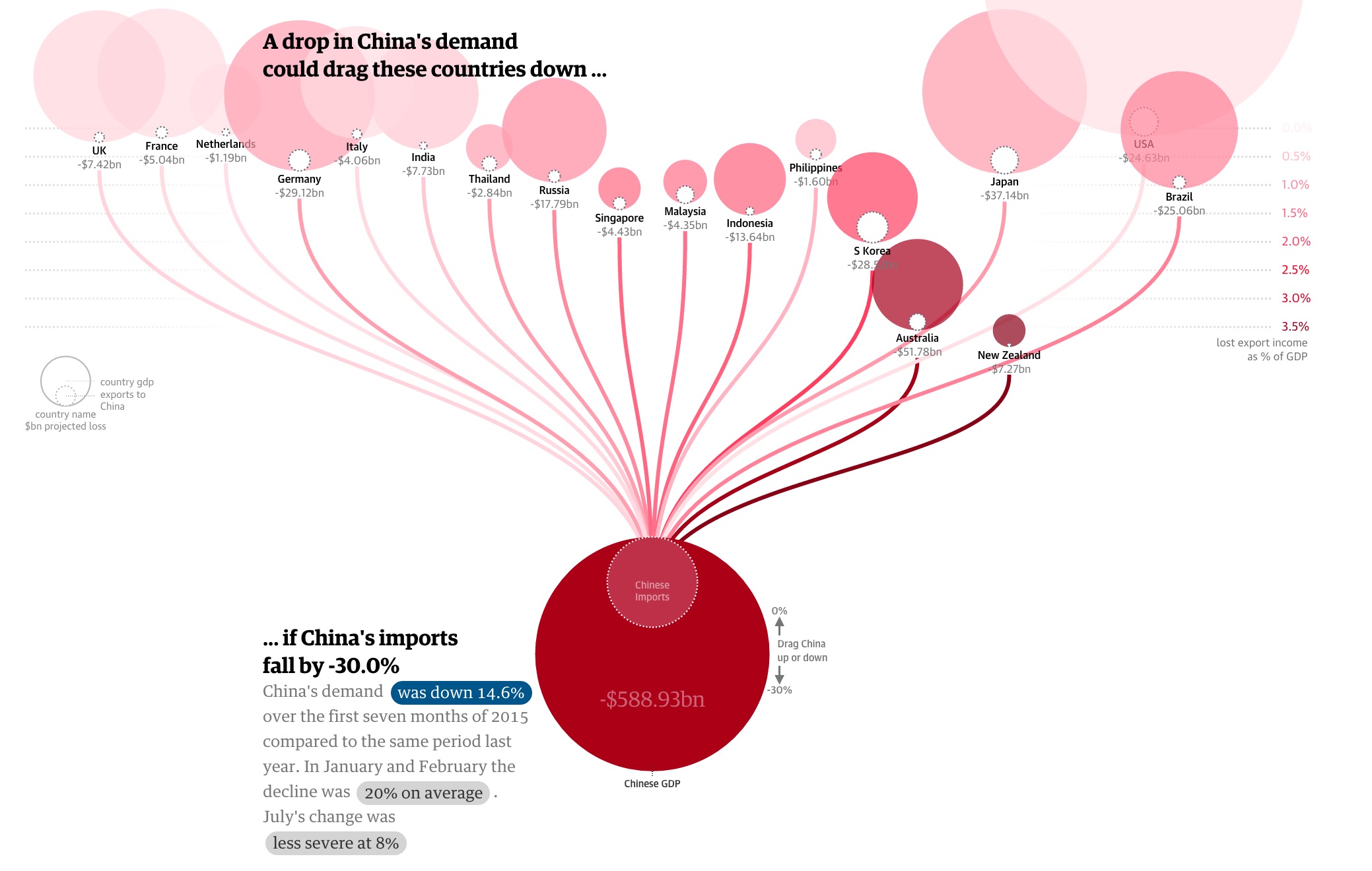
This is an interactive visualization of how 2015 China’s demand on import affects the economy of its trading partners. Indicated below, it is observed that the China’s growing momentum has started to slow down. To see how much China’s economy impacts the rest of the world, this visualization examined the relationship between China’s imports and other countries export.

The big dark red circle at the bottom represents China, and the inner circle represents China’s import demands. The China circle is connected to various trading partnering countries. By dragging the China circle up and down, we can manipulate the data to provision China’s import demand drop, from 0% to 30%, and we can observe the impact the change has on other countries shown by the export loss and its percentage of total GDP.

What I like about this

1. I like the interactivity aspect of this dashboard. Users can observe what impact China’s import demands has on its major trading partners.
2. The warrant of this visualization is that China is experiencing a slowdown in growth and as a result, its import demand decreases. The graph shows exactly how big of an impact it is to other countries. This is an effective way to show how China not only is a big exporting country but also an influential importing country.

What I don’t like about this

Overall, I think this is a very good visualization. However, there is one thing I find puzzling. The size of circles representing the export loss for China’s trading partners does not change when China’s import demand changes.

To represent the changes the countries experienced in regards to China’s import demands, this graph changed the location of the whole circle (representing each country). The more percentage of GDP loss, the lower the position of the whole circle (notice in the picture how low is Australia and New Zeland compare to others). Also, the more percentage of GDP loss, the darker the circle turns into. However, it took me a while to notice the relationship of the positioning and the % to GDP loss.

A user can also hover over each country, and the graph will show you the amount of money the country loss due to import demand decrease from China. I felt the size of the import loss should also change. For example, when China decreases import demand by 30%, the export loss of the US is at $24.63bn (0.1% GDP) and Australia at $51.78bn (3.6% GDP), but the circle representing loss in the US still remains significantly larger than the one representing the loss of Australia when in actuality, Australia will lose more than half of what the US will lose.

What I Would Have Done

1. Make the size of the export loss for each country change according to the amount of loss it will experiences when China’s import demand changes (as mentioned in the “What I don’t like about it” section).
2. I will also put a color scale indicator along with the visualization to indicate the darker the color the circle turned to means the heavier the impact because the current scale on the right-hand side looks like it just faded out at 0.0%

References

https://www.theguardian.com/world/ng-interactive/2015/aug/26/china-economic-slowdown-world-imports

China’s Economy Slow Down is Bad for America

The Ice Bucket Challenge, sometimes called the ALS Ice Bucket Challenge, is an activity involving the dumping of a bucket of ice and water over a person’s head, either by another person or self-administered, to promote awareness of the disease amyotrophic lateral sclerosis and encourage donations to research.

It went viral on social media during July–August 2014. The following visualization was trying to show how much money the ALS Ice Bucket Challenge has raised compared to how few die from the disease relative to other diseases.

There are 8 different diseases/causes considered, and each one is associated with a color. The sizes of the circles are proportional to the dollars raised for (on the left-hand side) and deaths caused by (on the right-hand side) the 8 diseases/causes. The graph looks pretty at first glance, but it suffers from the following problems:

What I like about it:

The colors are eye catching, and the bubbles are vivid.

What I don’t like about it:

1. Similar to pie charts, it is visually difficult to see the relative difference among diseases in the same category (deaths or dollars); readers are left guessing the relative sizes of the circles.
2. Because the dollars and deaths are not aligned by diseases, it forces the reader to look at one disease at a time; it is very difficult to spot a pattern between the 2 categories by diseases.
3. There are too many colors. I find myself going back and forth to the legend. It shouldn’t be so hard for the readers. Moreover, the colors are in no particular order; not alphabetical, not by deaths, nor not by money raised. This is way too confusing.
4. The font could be too small. The labels and number would be quite difficult to read from a distance.

 

Someone redid the graph, and came out with this dot chart above. It sure is easier to trace the relationship between the deaths and the money raised. But it still make it very difficult to illustrates the difference between the death tolls of diseases and the money raised to battle them.

In efficient visualization, we don’t need to present every detail information. On the contrary, we just need to point out our claim to the audience.

Re-creating the graph: 

The simple comparison line chart or bar chart will do a better job. Since we agreed in class that “function first, form follows”. This chart does a better job comparing the 2 categories by diseases than the bar charts with faceting. If we want to make sure that this chart is still functional for color blind people, we can minimize its color choices. “Get it right, Black & White.” I like how efficiently this minimalistic graph is able to convey the relevant information.

https://drive.google.com/file/d/0BwmDkc-M_2qyTjBESklxS2NuNnM/view?usp=sharing

(I uploaded the picture of the chart onto my google drive)

Conclusion:

In efficient visualization, a lot of times “less is more”. The first priority is find out the claim, and leave out the unnecessary information. ” Function first, form follows.”

References:

1. Makeover Monday: Where We Donate vs. Diseases that Kill Us

   http://www.vizwiz.com/2014/09/donations-vs-deaths.html

2. Redesign: Where We Donate vs. Diseases That Kill Us [OC]
3. https://www.reddit.com/r/dataisbeautiful/comments/2er3zq/redesign_where_we_donate_vs_diseases_that_kill_us/

Justin Mungal

Let’s face it, climate change is not just a debate, but a fierce fight for survival.  Those who reject 97% of scientists’ claims that human-driven carbon emissions are causing significant and catastrophic global warming are not merely “on the fence,” but rather vehemently opposed to what they categorize as conspiracy theory.  Any evidence that has more than a zero percent chance of speculation is utterly rejected by the group.  It is time to move the debate from scientific claim to scientific fact, where no ounce of speculation can be contorted into an “alternative fact.”

The journalists at Futurism have created “Five Graphics to Start a Conversation About Climate Change.” The first set of images depict what the majority of people believe, and that is that combined atmospheric temperatures are exponentially rising at alarming rates.  

While, this should be convincing enough, I no longer find it useful as climate change deniers claim that it represents normal fluctuations and that the correlation of rising CO2 emissions with these temperatures does not imply causation. This shred of speculation between correlation and causation collapses the debate into a stalemate, and so I believe that we must move the discussion into the realm of absolutely non-contentious facts.

The second set of images simply shows the rising rates of C02 emissions due to cement, gas, oil, and coal and its corresponding partitioning into the atmosphere and oceans.

This graphic is powerful because there is absolutely zero speculation and thus no room for debate.  Correlation and the (high) likelihood of causation are left off the table, and what remains is an impressive graphical representation of the massive amounts of human generated CO2 and its absorption into land, air and water.

The third graphic simply explains the science of how CO2 in the ocean can acidify its waters.

Again, there is no speculation of causation, it is merely a statement of scientific fact around the chemistry of water and CO2.  Effectively, this builds upon the second graphic, to raise the question of what impact our CO2 emissions can have on earth’s oceans.  The question is answered in the third graphic by the description of a chemical reaction summed up in the equation Dissolved C02 + Water à Carbonic Acid.  Again, there is no ambiguity or speculation – just solid scientific fact.

The fourth graphic shows how long C02 stays in the atmosphere after its initial pulse.

Seventy percent of pulsed C02 remains after one hundred years and forty percent remains after one thousand years.  Again, the graphic is not intended to show speculative correlation or causation, but rather clearly and accurately represents the fact of C02’s lifetime in the atmosphere.  Essentially, once CO2 is pulsed, it stays in the atmosphere for a very long time.  Coupled with graphics two and three, we see a picture of the massive amounts of C02 being emitted threatening the pH balance of our oceans for a long time.

The fifth graphic depicts projections of what earth’s climate might look like in the years 2081-2100.

https://futurism.com/wp-content/uploads/2017/05/5-climate-future-ipcc.jpg

The projections depict a boiling world of monsoon rains and ocean covered lands.  I could imagine that such a world would be barely, if at all, inhabitable by humans.  However, even I as a climate change believer, find this image difficult to digest.  I know that scientists find it difficult to predict the weather for a given week, so how accurate can hundred year projections be?  I do not deny that such predictions are possible considering our current global warming trends, but forecasting that far into the future seems spurious and, given the rash skepticism of the opposing side, non-provocative.

For the majority of us who believe in the work of climate scientists, graphics one and five are panic inducing.  We believe that the rising global temperatures are abnormal and humanly caused.  Moreover, the idea that the earth may not be humanly inhabitable for long if we continue on our current trajectory is not farfetched.  These two images capture that scientific consensus frighteningly well.  However, the purpose of this article, and I believe the necessary debate, is with those who reject such claims for the improbable claim that the overwhelming evidence of correlation does not imply causation.  That is why I am far fonder of graphics two, three, and four in terms of moving the debate forward.  They clearly and simply depict measurements and chemical reactions.  They cannot be negated as they do not contain any speculation over causation, are repeatable, and provable.  Thus, they can be starting points for serious debate over the current state of climate affairs and the ominous threats they imply.

What I would do to improve the graphics is include more visualizations like graphics two, three, and four.  Those engaged in the fight of their lives – the debate of climate change – need more ammo that cannot be misconstrued and discarded as circumstantial.  To spend more time creating images like graphics one and five are futile, as we know that the counterargument is to negate them as speculation and propaganda.    Unfortunately, we do not have time for visualizations whose validity is debatable – time is of the essence.

References:

<https://futurism.com/five-graphics-start-conversation-climate-change/>